7 Manipulating Data
Data-preprocessing is an important step in any data science process. Rarely will you receive data that is in the exact form that you need. More often than not, you would need to pre-process the data by transforming and manipulating them so that they are easier to work with. This will be the focus in this chapter.
7.1 Prerequisites
In this chapter we focus on the use of the dplyr package that forms a core part of the tidyverse package. dplyr provides function that alleviates the challenges of data manipulation.
To explore the basic data manipulation capabilities of dplyr package, we
will use the building_meter dataset. If the following code returns FALSE,
you should refer to the section Finding your file in the Preface on where
you can download the datasets.
This dataset contains 8,760 time-series observations of typical building meter measurements that is simulated using the Department of Energy’s (DOE) reference building energy model for medium sized offices [3].
bldg <- read_csv(here("data", "building_meter.csv"))
## Rows: 8760 Columns: 10
## ── Column specification ────────────────────────────────────────────────────────
## Delimiter: ","
## dbl  (9): Cooling:Electricity [J](Hourly), Heating:NaturalGas [J](Hourly), H...
## dttm (1): Date/Time
##
## ℹ Use `spec()` to retrieve the full column specification for this data.
## ℹ Specify the column types or set `show_col_types = FALSE` to quiet this message.
bldg
## # A tibble: 8,760 × 10
##    `Date/Time`         `Cooling:Electricity …` `Heating:Natur…` `Heating:Elect…`
##    <dttm>                                <dbl>            <dbl>            <dbl>
##  1 2020-01-01 01:00:00                       0        13517796.       182286476.
##  2 2020-01-01 02:00:00                       0        17717617.       177367416.
##  3 2020-01-01 03:00:00                       0        25310615.       235785509
##  4 2020-01-01 04:00:00                       0        20001989.       184762495.
##  5 2020-01-01 05:00:00                       0        27925599.       245249657.
##  6 2020-01-01 06:00:00                       0        21886933.       190670331.
##  7 2020-01-01 07:00:00                       0        29745424.       252272477.
....
Non-word characters such as spaces may make it difficult to reference columns. Therefore, a basic rule is to avoid naming columns using names that contain these characters in the first place. However, sometimes it is out of your control because you did not create the dataset but received it from source where the naming was done by someone else.
Take for example the building.csv data that we just parsed into R. names()
when applied to a data.frame() returns the column names of the data.frame
names(bldg)
##  [1] "Date/Time"
##  [2] "Cooling:Electricity [J](Hourly)"
##  [3] "Heating:NaturalGas [J](Hourly)"
##  [4] "Heating:Electricity [J](Hourly)"
##  [5] "InteriorLights:Electricity [J](Hourly)"
##  [6] "ExteriorLights:Electricity [J](Hourly)"
##  [7] "InteriorEquipment:Electricity [J](Hourly)"
##  [8] "Fans:Electricity [J](Hourly)"
##  [9] "Pumps:Electricity [J](Hourly)"
## [10] "WaterSystems:NaturalGas [J](Hourly)"
....
An easy way to remove non-word characters is to use the str_replace_all()
function to replace non-word characters with an underscore _. Referring back
to Chapter @ref{regex}, remember that \\W can be used to match non-word class
of characters while + is a quantifies that can be used to match a pattern one
or more times. Therefore, str_replace_all(names(bldg), "\\W+", "_") would
replace all non-word characters that appear one or more times in the character
vector names(bldg) with an underscore _.
new_name <- str_replace_all(names(bldg), "\\W+", "_")
new_name
##  [1] "Date_Time"
##  [2] "Cooling_Electricity_J_Hourly_"
##  [3] "Heating_NaturalGas_J_Hourly_"
##  [4] "Heating_Electricity_J_Hourly_"
##  [5] "InteriorLights_Electricity_J_Hourly_"
##  [6] "ExteriorLights_Electricity_J_Hourly_"
##  [7] "InteriorEquipment_Electricity_J_Hourly_"
##  [8] "Fans_Electricity_J_Hourly_"
##  [9] "Pumps_Electricity_J_Hourly_"
## [10] "WaterSystems_NaturalGas_J_Hourly_"
....
You can also remove parts of the character vector that you do not want using the
function str_remove_all().
names(bldg) <- str_remove_all(new_name, "_Hourly_")
names(bldg)
##  [1] "Date_Time"                       "Cooling_Electricity_J"
##  [3] "Heating_NaturalGas_J"            "Heating_Electricity_J"
##  [5] "InteriorLights_Electricity_J"    "ExteriorLights_Electricity_J"
##  [7] "InteriorEquipment_Electricity_J" "Fans_Electricity_J"
##  [9] "Pumps_Electricity_J"             "WaterSystems_NaturalGas_J"
7.2 Data transformation
The cheat sheet for dplyr provides a good summary of data transformation functions covered in this chapter.
-
select(): To select columns based on their names. -
filter(): To subset rows based on their values. -
mutate(): To add new variables whose values are a function of existing variables. -
arrange(): To sort the dataset based on the values of selected columns -
summarise()andgroup_by(): To apply computations by groups -
*_join(): generic functions that joins two tables together
7.2.1 select()
You can use the function select() to choose the variables to retain in the
dataset based on their names. It is not uncommon to get datasets with hundred or
thousands of variables. An example is when working with data from the building
management system. Under these scenarios, it is often very useful to narrow down
the dataset to contain only the variables of interest. select() allows you to
do this very easily, to zoom in on the variables or columns of interest.
select(bldg, Date_Time, Cooling_Electricity_J, Heating_Electricity_J)
## # A tibble: 8,760 × 3
##    Date_Time           Cooling_Electricity_J Heating_Electricity_J
##    <dttm>                              <dbl>                 <dbl>
##  1 2020-01-01 01:00:00                     0            182286476.
##  2 2020-01-01 02:00:00                     0            177367416.
##  3 2020-01-01 03:00:00                     0            235785509
##  4 2020-01-01 04:00:00                     0            184762495.
##  5 2020-01-01 05:00:00                     0            245249657.
##  6 2020-01-01 06:00:00                     0            190670331.
##  7 2020-01-01 07:00:00                     0            252272477.
....
You can also optionally rename columns with the select() function.
select(bldg,
    datetime = Date_Time,
    cooling = Cooling_Electricity_J,
    heating = Heating_Electricity_J
)
## # A tibble: 8,760 × 3
##    datetime            cooling    heating
##    <dttm>                <dbl>      <dbl>
##  1 2020-01-01 01:00:00       0 182286476.
##  2 2020-01-01 02:00:00       0 177367416.
##  3 2020-01-01 03:00:00       0 235785509
##  4 2020-01-01 04:00:00       0 184762495.
##  5 2020-01-01 05:00:00       0 245249657.
##  6 2020-01-01 06:00:00       0 190670331.
##  7 2020-01-01 07:00:00       0 252272477.
....
Additionally, tidyverse provides helper functions that lets you select columns
by matching patterns in their names. For the following selection helper
functions, a character vector is provided for the match. If length() of the
character vector is larger than 1, the logical union (OR | operator) is taken.
-
starts_with(): Select columns that starts with a specific character vector
select(bldg, starts_with(c("Heating", "Cooling")))
## # A tibble: 8,760 × 3
##    Heating_NaturalGas_J Heating_Electricity_J Cooling_Electricity_J
##                   <dbl>                 <dbl>                 <dbl>
##  1            13517796.            182286476.                     0
##  2            17717617.            177367416.                     0
##  3            25310615.            235785509                      0
##  4            20001989.            184762495.                     0
##  5            27925599.            245249657.                     0
##  6            21886933.            190670331.                     0
##  7            29745424.            252272477.                     0
....-
ends_with(): Select columns that ends with a specific character vector
select(bldg, ends_with("Time"))
## # A tibble: 8,760 × 1
##    Date_Time
##    <dttm>
##  1 2020-01-01 01:00:00
##  2 2020-01-01 02:00:00
##  3 2020-01-01 03:00:00
##  4 2020-01-01 04:00:00
##  5 2020-01-01 05:00:00
##  6 2020-01-01 06:00:00
##  7 2020-01-01 07:00:00
....-
contains(): Select columns that contains a specific character vector
select(
    bldg,
    contains(
        c(
            "Time",
            "electricity"
        )
    )
)
## # A tibble: 8,760 × 8
##    Date_Time           Cooling_Electricity_J Heating_Electrici… InteriorLights_…
##    <dttm>                              <dbl>              <dbl>            <dbl>
##  1 2020-01-01 01:00:00                     0         182286476.         9649498.
##  2 2020-01-01 02:00:00                     0         177367416.         9649498.
##  3 2020-01-01 03:00:00                     0         235785509          9649498.
##  4 2020-01-01 04:00:00                     0         184762495.         9649498.
##  5 2020-01-01 05:00:00                     0         245249657.         9649498.
##  6 2020-01-01 06:00:00                     0         190670331.         9649498.
##  7 2020-01-01 07:00:00                     0         252272477.         9649498.
....-
matches(): Select columns that matches a regular expression.rename()is a dplyr function that allows you to change the names of individual columns usingnew_name=old_name. Referring back to Chapter [regex], remember that the.is used to match any character except newline\nwhile?is a quantifier that can be used to match a pattern zero or one times.
reg_ex <- "[dD]ate.?[tT]ime"

select(bldg, matches(reg_ex, ignore.case = FALSE))
## # A tibble: 8,760 × 1
##    Date_Time
##    <dttm>
##  1 2020-01-01 01:00:00
##  2 2020-01-01 02:00:00
##  3 2020-01-01 03:00:00
##  4 2020-01-01 04:00:00
##  5 2020-01-01 05:00:00
##  6 2020-01-01 06:00:00
##  7 2020-01-01 07:00:00
....

bldg_rename_a <- rename(bldg, `Date/Time` = `Date_Time`)
select(bldg_rename_a, matches(reg_ex, ignore.case = FALSE))
## # A tibble: 8,760 × 1
##    `Date/Time`
##    <dttm>
##  1 2020-01-01 01:00:00
##  2 2020-01-01 02:00:00
##  3 2020-01-01 03:00:00
##  4 2020-01-01 04:00:00
##  5 2020-01-01 05:00:00
##  6 2020-01-01 06:00:00
##  7 2020-01-01 07:00:00
....


bldg_rename_b <- rename(bldg, `datetime` = `Date_Time`)
select(bldg_rename_b, matches(reg_ex, ignore.case = FALSE))
## # A tibble: 8,760 × 1
##    datetime
##    <dttm>
##  1 2020-01-01 01:00:00
##  2 2020-01-01 02:00:00
##  3 2020-01-01 03:00:00
##  4 2020-01-01 04:00:00
##  5 2020-01-01 05:00:00
##  6 2020-01-01 06:00:00
##  7 2020-01-01 07:00:00
....-
all_of()andany_of(): You can also select variables from a character vector using the selection helper functionsall_of()andany_of(). The key difference is thatall_of()is used for strict selection where an error is thrown for variable names that do not exist. In contrast,any_of()does not check for missing variable names, and thus is often used to ensure a specific column is removed.
vars <- c("Heating_NaturalGas_J", "WaterSystems_NaturalGas_J")
select(bldg, all_of(vars))
## # A tibble: 8,760 × 2
##    Heating_NaturalGas_J WaterSystems_NaturalGas_J
##                   <dbl>                     <dbl>
##  1            13517796.                    72000
##  2            17717617.                    72000
##  3            25310615.                  3970732.
##  4            20001989.                    72000
##  5            27925599.                  3970995.
##  6            21886933.                    72000
##  7            29745424.                  3970782.
....

select(bldg, -any_of(vars))
## # A tibble: 8,760 × 8
##    Date_Time           Cooling_Electricity_J Heating_Electrici… InteriorLights_…
##    <dttm>                              <dbl>              <dbl>            <dbl>
##  1 2020-01-01 01:00:00                     0         182286476.         9649498.
##  2 2020-01-01 02:00:00                     0         177367416.         9649498.
##  3 2020-01-01 03:00:00                     0         235785509          9649498.
##  4 2020-01-01 04:00:00                     0         184762495.         9649498.
##  5 2020-01-01 05:00:00                     0         245249657.         9649498.
##  6 2020-01-01 06:00:00                     0         190670331.         9649498.
##  7 2020-01-01 07:00:00                     0         252272477.         9649498.
....-
where()is a very useful selection helper function when you want to apply a function (that returnsTRUEorFALSE) to all columns and select only those columns where the function returnsTRUE.
select(bldg, where(is.numeric))
## # A tibble: 8,760 × 9
##    Cooling_Electricity_J Heating_NaturalGas_J Heating_Electric… InteriorLights_…
##                    <dbl>                <dbl>             <dbl>            <dbl>
##  1                     0            13517796.        182286476.         9649498.
##  2                     0            17717617.        177367416.         9649498.
##  3                     0            25310615.        235785509          9649498.
##  4                     0            20001989.        184762495.         9649498.
##  5                     0            27925599.        245249657.         9649498.
##  6                     0            21886933.        190670331.         9649498.
##  7                     0            29745424.        252272477.         9649498.
....
You can also define the function to be applied within where()
select(
    bldg,
    where(
        function(x) is.numeric(x)
    )
)
## # A tibble: 8,760 × 9
##    Cooling_Electricity_J Heating_NaturalGas_J Heating_Electric… InteriorLights_…
##                    <dbl>                <dbl>             <dbl>            <dbl>
##  1                     0            13517796.        182286476.         9649498.
##  2                     0            17717617.        177367416.         9649498.
##  3                     0            25310615.        235785509          9649498.
##  4                     0            20001989.        184762495.         9649498.
##  5                     0            27925599.        245249657.         9649498.
##  6                     0            21886933.        190670331.         9649498.
##  7                     0            29745424.        252272477.         9649498.
....
7.2.2 filter()
You can use filter() to subset rows based on their values. {dplyr}'s
filter() function retains rows that return TRUE for all the conditions
specified. The first argument is the data frame and the subsequent arguments are
the conditions that are used to subset the observations. In other words,
multiple arguments to filter() are combined by the & (and) logical operator.
To work with other logical operators such as | (or) and ! (not), you would
have to combine them within a single argument.
filter(bldg, Cooling_Electricity_J != 0)
## # A tibble: 2,678 × 10
##    Date_Time           Cooling_Electricity_J Heating_NaturalGa… Heating_Electri…
##    <dttm>                              <dbl>              <dbl>            <dbl>
##  1 2020-02-11 15:00:00              4354833.                  0        91807743.
##  2 2020-02-11 16:00:00              2387624.                  0        94118327.
##  3 2020-02-23 09:00:00              7606370.                  0       102607149.
##  4 2020-02-23 10:00:00             21074975.                  0        76304715.
##  5 2020-02-23 11:00:00             23052733.                  0        63182232.
##  6 2020-02-23 12:00:00             23185185.                  0        53130886.
##  7 2020-02-23 13:00:00             20501352.                  0        68037068.
....

filter(bldg, InteriorLights_Electricity_J > 100000000)
## # A tibble: 2,520 × 10
##    Date_Time           Cooling_Electricity_J Heating_NaturalGa… Heating_Electri…
##    <dttm>                              <dbl>              <dbl>            <dbl>
##  1 2020-01-02 09:00:00                     0         128483630.       473529413.
##  2 2020-01-02 10:00:00                     0         109562756.       398893378.
##  3 2020-01-02 11:00:00                     0          88363562.       350234124.
##  4 2020-01-02 12:00:00                     0          75198754.       305357974
##  5 2020-01-02 13:00:00                     0          70573992.       300958898.
##  6 2020-01-02 14:00:00                     0          84277786.       249050033.
##  7 2020-01-02 15:00:00                     0          99713290.       238506555.
....

filter(
    bldg, Cooling_Electricity_J != 0,
    Cooling_Electricity_J < 4000000 |
        Cooling_Electricity_J > 22000000,
)
## # A tibble: 2,428 × 10
##    Date_Time           Cooling_Electricity_J Heating_NaturalGa… Heating_Electri…
##    <dttm>                              <dbl>              <dbl>            <dbl>
##  1 2020-02-11 16:00:00              2387624.                  0        94118327.
##  2 2020-02-23 11:00:00             23052733.                  0        63182232.
##  3 2020-02-23 12:00:00             23185185.                  0        53130886.
##  4 2020-02-23 20:00:00              1387715.                  0       101207501.
##  5 2020-03-10 12:00:00             25148879.                  0        17802883.
##  6 2020-03-10 13:00:00             31261163.                  0        15048079.
##  7 2020-03-10 14:00:00             30172661.                  0         1791300.
....
Often, the ability to subset observations based on their timestamp is a very useful feature when working with timeseries data
filter(bldg, month(Date_Time) == 1, day(Date_Time) == 1)
## # A tibble: 24 × 10
##    Date_Time           Cooling_Electricity_J Heating_NaturalGa… Heating_Electri…
##    <dttm>                              <dbl>              <dbl>            <dbl>
##  1 2020-01-01 01:00:00                     0          13517796.       182286476.
##  2 2020-01-01 02:00:00                     0          17717617.       177367416.
##  3 2020-01-01 03:00:00                     0          25310615.       235785509
##  4 2020-01-01 04:00:00                     0          20001989.       184762495.
##  5 2020-01-01 05:00:00                     0          27925599.       245249657.
##  6 2020-01-01 06:00:00                     0          21886933.       190670331.
##  7 2020-01-01 07:00:00                     0          29745424.       252272477.
....

filter(bldg, day(Date_Time) == 1)
## # A tibble: 287 × 10
##    Date_Time           Cooling_Electricity_J Heating_NaturalGa… Heating_Electri…
##    <dttm>                              <dbl>              <dbl>            <dbl>
##  1 2020-01-01 01:00:00                     0          13517796.       182286476.
##  2 2020-01-01 02:00:00                     0          17717617.       177367416.
##  3 2020-01-01 03:00:00                     0          25310615.       235785509
##  4 2020-01-01 04:00:00                     0          20001989.       184762495.
##  5 2020-01-01 05:00:00                     0          27925599.       245249657.
##  6 2020-01-01 06:00:00                     0          21886933.       190670331.
##  7 2020-01-01 07:00:00                     0          29745424.       252272477.
....

filter(bldg, month(Date_Time) > 4, month(Date_Time) < 10)
## # A tibble: 3,672 × 10
##    Date_Time           Cooling_Electricity_J Heating_NaturalGa… Heating_Electri…
##    <dttm>                              <dbl>              <dbl>            <dbl>
##  1 2020-05-01 00:00:00                    0                   0               0
##  2 2020-05-01 01:00:00                    0                   0               0
##  3 2020-05-01 02:00:00                    0                   0               0
##  4 2020-05-01 03:00:00                    0                   0               0
##  5 2020-05-01 04:00:00                    0                   0               0
##  6 2020-05-01 05:00:00                    0                   0               0
##  7 2020-05-01 06:00:00                    0                   0       252935532.
....

filter(bldg, month(Date_Time) > 4 & month(Date_Time) < 10)
## # A tibble: 3,672 × 10
##    Date_Time           Cooling_Electricity_J Heating_NaturalGa… Heating_Electri…
##    <dttm>                              <dbl>              <dbl>            <dbl>
##  1 2020-05-01 00:00:00                    0                   0               0
##  2 2020-05-01 01:00:00                    0                   0               0
##  3 2020-05-01 02:00:00                    0                   0               0
##  4 2020-05-01 03:00:00                    0                   0               0
##  5 2020-05-01 04:00:00                    0                   0               0
##  6 2020-05-01 05:00:00                    0                   0               0
##  7 2020-05-01 06:00:00                    0                   0       252935532.
....
You can also combine filter() with grepl() to subset rows using regular
expressions.
7.2.3 arrange()
You can use arrange() to sort the dataset based on the values of selected
columns. The first argument is the data frame and the second is the column name
to sort the data frame by. If more than one column name is provided, subsequent
column names will be used to break ties in the preceding columns.
arrange(bldg, Cooling_Electricity_J)
## # A tibble: 8,760 × 10
##    Date_Time           Cooling_Electricity_J Heating_NaturalGa… Heating_Electri…
##    <dttm>                              <dbl>              <dbl>            <dbl>
##  1 2020-01-01 01:00:00                     0          13517796.       182286476.
##  2 2020-01-01 02:00:00                     0          17717617.       177367416.
##  3 2020-01-01 03:00:00                     0          25310615.       235785509
##  4 2020-01-01 04:00:00                     0          20001989.       184762495.
##  5 2020-01-01 05:00:00                     0          27925599.       245249657.
##  6 2020-01-01 06:00:00                     0          21886933.       190670331.
##  7 2020-01-01 07:00:00                     0          29745424.       252272477.
....
You can use desc() to order a column in descending order
arrange(bldg, desc(Cooling_Electricity_J))
## # A tibble: 8,760 × 10
##    Date_Time           Cooling_Electricity_J Heating_NaturalGa… Heating_Electri…
##    <dttm>                              <dbl>              <dbl>            <dbl>
##  1 2020-07-19 16:00:00            356330907.                  0                0
##  2 2020-07-19 15:00:00            349038364.                  0                0
##  3 2020-07-18 16:00:00            339376366.                  0                0
##  4 2020-07-19 17:00:00            338918865.                  0                0
##  5 2020-07-17 15:00:00            337245696.                  0                0
##  6 2020-07-18 14:00:00            336127683.                  0                0
##  7 2020-07-17 16:00:00            335013419.                  0                0
....
7.2.4 mutate()
You can use mutate() to add new variables whose values are a function of
existing variables (Note that you can also refer to newly created variables).
The newly created variables will be added to the end of the dataset.
mutate(bldg,
    Total_Heating_J = Heating_NaturalGas_J + Heating_Electricity_J,
    Cooling_Heating_kWh = (Total_Heating_J + Cooling_Electricity_J) * 2.77778e-7
)
## # A tibble: 8,760 × 12
##    Date_Time           Cooling_Electricity_J Heating_NaturalGa… Heating_Electri…
##    <dttm>                              <dbl>              <dbl>            <dbl>
##  1 2020-01-01 01:00:00                     0          13517796.       182286476.
##  2 2020-01-01 02:00:00                     0          17717617.       177367416.
##  3 2020-01-01 03:00:00                     0          25310615.       235785509
##  4 2020-01-01 04:00:00                     0          20001989.       184762495.
##  5 2020-01-01 05:00:00                     0          27925599.       245249657.
##  6 2020-01-01 06:00:00                     0          21886933.       190670331.
##  7 2020-01-01 07:00:00                     0          29745424.       252272477.
....
You can use transmute() if you only want to keep the new variables in your
dataset.
transmute(bldg,
    Total_Heating_J = Heating_NaturalGas_J + Heating_Electricity_J,
    Cooling_Heating_kWh = (Total_Heating_J + Cooling_Electricity_J) * 2.77778e-7
)
## # A tibble: 8,760 × 2
##    Total_Heating_J Cooling_Heating_kWh
##              <dbl>               <dbl>
##  1      195804272.                54.4
##  2      195085034.                54.2
##  3      261096124.                72.5
##  4      204764484.                56.9
##  5      273175257.                75.9
##  6      212557265.                59.0
##  7      282017901.                78.3
....
Useful mutate and transmute functions include
heat <- transmute(bldg,
    Total_Heating_J = Heating_NaturalGas_J + Heating_Electricity_J
)
heat
## # A tibble: 8,760 × 1
##    Total_Heating_J
##              <dbl>
##  1      195804272.
##  2      195085034.
##  3      261096124.
##  4      204764484.
##  5      273175257.
##  6      212557265.
##  7      282017901.
....-
lead()andlag(), allowing you to create lead and lag variables that are useful especially when working with timeseries data.
mutate(
    heat,
    lag_1 = lag(Total_Heating_J),
    lag_2 = lag(lag_1),
    lag_3 = lag(Total_Heating_J, 3)
)
## # A tibble: 8,760 × 4
##    Total_Heating_J      lag_1      lag_2      lag_3
##              <dbl>      <dbl>      <dbl>      <dbl>
##  1      195804272.        NA         NA         NA
##  2      195085034. 195804272.        NA         NA
##  3      261096124. 195085034. 195804272.        NA
##  4      204764484. 261096124. 195085034. 195804272.
##  5      273175257. 204764484. 261096124. 195085034.
##  6      212557265. 273175257. 204764484. 261096124.
##  7      282017901. 212557265. 273175257. 204764484.
....-
if_else()is function of the formif_else(condition, true, false)that allows you to test a condition that you provide as a first argument to the function. If the condition isTRUE,if_else()will return the second argument. By contrast, if the condition isFALSE, it will return the third argument. In the example below, we are using mutate to create a new variable/columnNew_Total_Heating_J. This new column will contain the characters"low"if the conditionTotal_Heating_J < 200000000isTRUEand"high"if it isFALSE.
mutate(
    heat,
    New_Total_Heating_J = if_else(Total_Heating_J < 200000000, "low", "high")
)
## # A tibble: 8,760 × 2
##    Total_Heating_J New_Total_Heating_J
##              <dbl> <chr>
##  1      195804272. low
##  2      195085034. low
##  3      261096124. high
##  4      204764484. high
##  5      273175257. high
##  6      212557265. high
##  7      282017901. high
....-
case_when()is an extension ofif_else()by allowing you to write multipleif_else()statements. Below, we assign a"low"whenTotal_Heating_J < 200000000,"medium"when200000000 <= Total_Heating_J <= 400000000, and high whenTotal_Heating_J > 400000000.
mutate(
    heat,
    New_Total_Heating_J = case_when(
        Total_Heating_J < 200000000 ~ "low",
        Total_Heating_J >= 200000000 & Total_Heating_J <= 400000000 ~ "medium",
        Total_Heating_J > 400000000 ~ "high"
    )
)
## # A tibble: 8,760 × 2
##    Total_Heating_J New_Total_Heating_J
##              <dbl> <chr>
##  1      195804272. low
##  2      195085034. low
##  3      261096124. medium
##  4      204764484. medium
##  5      273175257. medium
##  6      212557265. medium
##  7      282017901. medium
....
7.2.5 summarise() and group_by()
summarise() or summarize() collapse a data frame into one row for each
combination of grouping variables. Therefore, it is not very useful by itself.
summarise(bldg,
    Heating_Total = sum(Heating_Electricity_J),
    Heating_Avg = mean(Heating_Electricity_J),
    Heating_Peak = max(Heating_Electricity_J)
)
## # A tibble: 1 × 3
##   Heating_Total Heating_Avg Heating_Peak
##           <dbl>       <dbl>        <dbl>
## 1 508713824519.   58072354.   1002989103
However, summarise() combined with group_by() will allow you to easily
summarise data based on individual groups.
bldg_month <- mutate(bldg,
    Year = year(Date_Time),
    Month = month(Date_Time)
)

bldg_by_month <- group_by(bldg_month, Year, Month)

summarise(bldg_by_month,
    Heating_Total = sum(Heating_Electricity_J),
    Heating_Avg = mean(Heating_Electricity_J),
    Heating_Peak = max(Heating_Electricity_J)
)
## `summarise()` has grouped output by 'Year'. You can override using the
## `.groups` argument.
## # A tibble: 13 × 5
## # Groups:   Year [2]
##     Year Month Heating_Total Heating_Avg Heating_Peak
##    <dbl> <dbl>         <dbl>       <dbl>        <dbl>
##  1  2020     1 124527837066.  167601396.   978585992.
##  2  2020     2  89836688374.  133486907.  1002989103
##  3  2020     3  55674915533.   74932592.   795581602.
##  4  2020     4  32036849861.   44495625.   639342141.
##  5  2020     5   7726081874.   10384519.   252935532.
##  6  2020     6    624415414.     867244.    39920827.
....
7.2.6 across()
across() makes it possible to apply functions across multiple columns within
the functions summarise() and mutate(), using the semantics in filter()
(see section 7.2.1) that makes it easy to refer to columns based on
their names.
transmute(bldg,
    Date_Time,
    total = rowSums(across(where(is.numeric)))
)
## # A tibble: 8,760 × 2
##    Date_Time                total
##    <dttm>                   <dbl>
##  1 2020-01-01 01:00:00 326555010.
##  2 2020-01-01 02:00:00 324420893.
##  3 2020-01-01 03:00:00 396428863.
##  4 2020-01-01 04:00:00 334100344.
##  5 2020-01-01 05:00:00 408508259.
##  6 2020-01-01 06:00:00 341893124.
##  7 2020-01-01 07:00:00 417350691.
....
You may also pass a list of functions to be applied to each of the selected columns.
summarise(
    bldg_by_month,
    across(
        contains("electricity"),
        list(Total = sum, Avg = mean, Peak = max)
    )
)
## `summarise()` has grouped output by 'Year'. You can override using the
## `.groups` argument.
## # A tibble: 13 × 23
## # Groups:   Year [2]
##     Year Month Cooling_Electricity_J_Total Cooling_Electricity… Cooling_Electri…
##    <dbl> <dbl>                       <dbl>                <dbl>            <dbl>
##  1  2020     1                          0                    0                0
##  2  2020     2                  181014017.              268966.        23185185.
##  3  2020     3                  775169988.             1043297.        79053134.
##  4  2020     4                11551697867.            16044025.       226399417.
##  5  2020     5                22952133253.            30849641.       191404162.
##  6  2020     6                53405646191.            74174509.       302585966
....
7.3 Pipes
The %>% is a forward pipe operator from the magrittr package that comes
loaded with the tidyverse package. The pipe operator %>% is a very handy
that allows operations to be performed sequentially. In general, you can think
of it as sending the output of one function as an input to the next .
With the pipe operator,
Instead of many intermediary steps
first_output <- first(data)
second_output <- second(first_output)
final_result <- third(second_output)
You can connect multiple operators sequentially using the pipe operator
Figure 7.1 shows what is happening graphically.
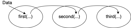
Figure 7.1: Piping data from one function to the next sequentially
An example using the bldg dataset.
bldg %>%
    select(Date_Time, contains("Heating")) %>%
    mutate(
        Month = month(Date_Time),
        Total_Heating_J = rowSums(across(where(is.numeric)))
    ) %>%
    group_by(Month) %>%
    summarise(across(
        where(is.numeric),
        list(Total = sum, Peak = max)
    ))
## # A tibble: 12 × 7
##    Month Heating_NaturalGas_… Heating_Natural… Heating_Electri… Heating_Electri…
##    <dbl>                <dbl>            <dbl>            <dbl>            <dbl>
##  1     1         59660445562.       527825997.    124648935250.       978585992.
##  2     2         41029360544.       530570172.     89836688374.      1002989103
##  3     3          9377325423.       230991815.     55674915533.       795581602.
##  4     4          3352997015.       156525821      32036849861.       639342141.
##  5     5             2144014.         2144014.      7726081874.       252935532.
##  6     6                   0                0        624415414.        39920827.
##  7     7                   0                0        128302310.        16757642
....