16 Model Exploration

16.1 Prerequisites

In this chapter we will explore the model to uncover energy characteristics and create an overview of general trends. We will use eplusr to run the EnergyPlus simulation and extract relevant model inputs/outputs, tidyverse for data transformation, and ggplot2 to visualize the extracted and subsequently transformed data.

library(eplusr)
library(tidyverse)
library(lubridate)
library(ggplot2)
library(here)

We will be working with the IDF and EPW file that pertains to the U.S. Department of Energy (DOE) Commercial Reference Building and Chicago’s TMY3 respectively.

path_idf <- here("data", "idf", "RefBldgMediumOfficeNew2004_Chicago.idf")
model <- read_idf(path_idf)

path_epw <- here("data", "epw", "USA_IL_Chicago-OHare.Intl.AP.725300_TMY3.epw")
epw <- read_epw(path_epw)

16.2 Extracting

Before carrying out any model exploration, you need to first specify the outputs of interest. The code below preprocesses the model by adding the list of output meters and variables to the model (See Chapter 15 for details).

preprocess_idf <- function(idf, meters, variables) {
    # make sure weather file input is respected
    idf$SimulationControl$Run_Simulation_for_Weather_File_Run_Periods <- "Yes"

    # make sure simulation is not run for sizing periods
    idf$SimulationControl$Run_Simulation_for_Sizing_Periods <- "No"

    # make sure energy consumption is presented in kWh
    if (is.null(idf$OutputControl_Table_Style)) {
        idf$add(OutputControl_Table_Style = list("HTML", "JtoKWH"))
    } else {
        idf$OutputControl_Table_Style$Unit_Conversion <- "JtoKWH"
    }

    # remove all existing meter and variable outputs
    if (!is.null(idf$`Output:Meter`)) {
        idf$Output_Meter <- NULL
    }

    # remove all existing meter and variable outputs
    if (!is.null(idf$`Output:Table:Monthly`)) {
        idf$`Output:Table:Monthly` <- NULL
    }

    if (!is.null(idf$`Output:Variable`)) {
        idf$Output_Variable <- NULL
    }

    # add meter outputs to get hourly time-series energy consumption
    idf$add(Output_Meter := meters)

    # add variable outputs to get hourly zone air temperature
    idf$add(Output_Variable := variables)

    # make sure the modified model is returned
    return(idf)
}

meters <- list(
    key_name = c(
        "Cooling:Electricity",
        "Heating:NaturalGas",
        "Heating:Electricity",
        "InteriorLights:Electricity",
        "ExteriorLights:Electricity",
        "InteriorEquipment:Electricity",
        "Fans:Electricity",
        "Pumps:Electricity",
        "WaterSystems:NaturalGas"
    ),
    Reporting_Frequency = "Hourly"
)

variables <- list(
    key_value = "*",
    Variable_Name = c(
        "Site Outdoor Air Drybulb Temperature",
        "Site Outdoor Air Relative Humidity"
    ),
    Reporting_Frequency = "Hourly"
)

model <- preprocess_idf(model, meters, variables)

You can then run the simulation and it will be possible to extract the output of interest from the model.

model$save(here("data", "idf", "model_preprocessed.idf"), overwrite = TRUE)
## Replace the existing IDF located at /home/runner/work/r4bes/r4bes/data/idf/model_preprocessed.idf.
job <- model$run(epw, dir = tempdir())
## ExpandObjects Started.
## No expanded file generated.
## ExpandObjects Finished. Time:     0.051
## EnergyPlus Starting
## EnergyPlus, Version 9.4.0-998c4b761e, YMD=2023.03.09 00:29
## Could not find platform independent libraries <prefix>
## Could not find platform dependent libraries <exec_prefix>
## Consider setting $PYTHONHOME to <prefix>[:<exec_prefix>]
## 
## Initializing Response Factors
## Calculating CTFs for "STEEL FRAME NON-RES EXT WALL"
## Calculating CTFs for "IEAD NON-RES ROOF"
## Calculating CTFs for "EXT-SLAB"
## Calculating CTFs for "INT-WALLS"
## Calculating CTFs for "INT-FLOOR-TOPSIDE"
....

16.3 Energy signature

pt_of_interest <- c(
    "Site Outdoor Air Drybulb Temperature",
    "Cooling:Electricity",
    "Heating:NaturalGas"
)

report <- job$report_data(
        name = pt_of_interest, environment_name = "annual",
        all = TRUE, wide = TRUE
    ) %>%
    select(datetime, month, day, hour, day_type, contains(pt_of_interest)) %>%
    rename_with(~pt_of_interest, .cols = contains(pt_of_interest)) %>%
    pivot_longer(
        cols = c("Cooling:Electricity", "Heating:NaturalGas"),
        names_to = "type", values_to = "value"
    ) %>%
    mutate(
        value = value * 1e-6, # convert J to MJ
        month = ordered(month.abb[month], month.abb) # replace month index with month name
    )

ggplot(report, aes(
    x = `Site Outdoor Air Drybulb Temperature`,
    y = value,
    color = type
)) +
    geom_point(shape = 1, alpha = 0.7) +
    facet_grid(rows = vars(type)) +
    scale_color_brewer(palette = "Set2") +
    xlab(expression("Outdoor drybulb temperature" ~ (degree * C))) +
    ylab("Energy consumption (MJ)") +
    theme(legend.position = "none")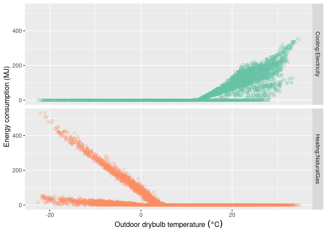

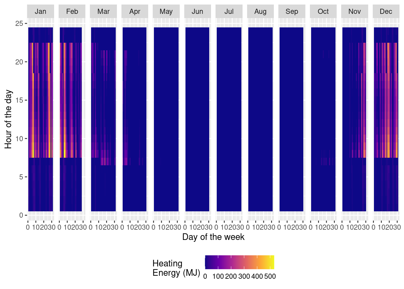
report_heating <- report %>%
    filter(type == "Heating:NaturalGas")

ggplot(report_heating, aes(
    x = day, y = hour,
    fill = value
)) +
    geom_tile() +
    scale_fill_viridis_c(
        name = "Heating\nEnergy (MJ)",
        option = "plasma"
    ) +
    facet_grid(cols = vars(month)) +
    ylab("Hour of the day") +
    xlab("Day of the week") +
    theme(legend.position = "bottom")